3.3 Logarithmic Functions

Introduction

Up until the invention of scientific calculators 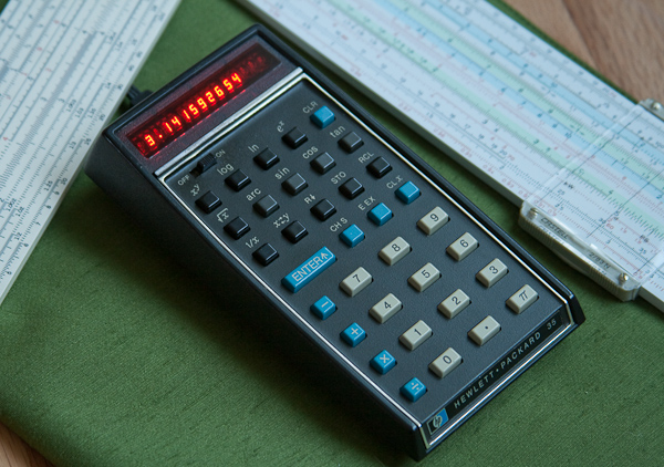The HP-35 was the first handheld scientific calculator. Developed by Hewlett-Packard, it went on sale in 1972 for $395. Photo by Julian Bucknall in the 1970's, people relied on 300-year-old mechanical calculators called "slide rules".

Slide rules use the properties of exponents to simplify calculations. For example, multiplication turns into addition and division becomes subtraction.

To build a slide rule you need a function that can extract exponents. Such functions are called logarithmic functions and just happen to be the inverses of exponential functions. In this section we will study logarithms and even learn how to use a simple slide rule.

Definition of Logarithms

We learned in a previous chapter that every one-to-one function has an inverse. Since the exponential function $b^{x}$ (where $b>0$ and $b\neq1$) is one-to-one, it must have an inverse.

The inverse of the exponential with base $b$ is called the logarithm with base $b$ and is written $\log_b (x)$.

As with exponential functions, the base $b$ must be a positive number not equal to $1$.

In other words, as long as the base is the same, the functions $b^{x}$ and $\log_b(x)$ are inverses of each other.

Function	Inverse
$f(x) = 3^{x}$	Answer $f^{-1}(x) = \log_{3}(x)$
$g(x) = \log_{4} (x)$	Answer $g^{-1}(x) = 4^{x}$
$h(t) = 2^t$	Answer $h^{-1}(t) = \log_2(t)$
$q(x) = \log_{10}(x)$	Answer $q^{-1}(x) = 10^{x}$

Convert Between Exponential and Logarithmic Equations

Whenever a function has an inverse, we know that $f(x) = y$ if and only if $f^{-1}(y) = x$. In the present context, this inverse relationship means that $y = b^{x}$ is equivalent to $\log_{b}(y) = x$.

This gives us the ability to rewrite exponential equations as logarithmic equations and/or convert logarithmic equations into exponential equations. To convert between exponential and logarithmic equations it is easiest to first identify the base and then remember that the logarithm equals the exponent.

For example, the exponential equation $9=3^{2}$ is equivalent to logarithmic equation $\log_{3}(9) = 2$.

Going the other direction, $\log_{10}(1000)=3$ means the same thing as $1000=10^{3}$. Here are a few more examples.

	Exponential Equation	Logarithmic Equation
a.	$5^{3}=125$	Answer $\log_{5}125=3$
b.	$9^{2}=81$	Answer $\log_{9}81=2$
c.	$3^{y}=4$	Answer $y=\log_{3}4$
d.	Answer $2^4=16$	$\log_2(16)=4$
e.	Answer $3^{3}=27$	$\log_3(27)=3$
f.	Answer $10^5=x$	$\log_{10}(x)=5$

Evaluate Logarithms

The inverse relationship

[ y=b^{x} \Longleftrightarrow \log_{b}(y) = x ]

can also be used to evaluate logarithms by rewriting known exponential values. To illustrate this point, let's compute a few values of $\log_{2}(x)$ by looking at known values of $2^{x}$.

$y=2^{x} \Longleftrightarrow \log_{2}(y)=$	$x$
$1=2^{0} \Longleftrightarrow \log_{2}(1)=$	Answer $0$
$2=2^{1} \Longleftrightarrow \log_{2}(2)=$	Answer $1$
$4=2^{2} \Longleftrightarrow \log_{2}(4)=$	Answer $2$
$8=2^{3} \Longleftrightarrow \log_{2}(8)=$	Answer $3$

Notice that in each instance the logarithm is the exponent. For example, $\log_{2}(8)=3$ because $3$ is the exponent that makes $2^{x}=8$.

Of course, logarithmic functions can also be evaluated on a calculator. Starting with the HP-35 in 1972, two different logarithms have been built into every handheld scientific and graphing calculator: the common log and the natural log. The buttons for $\log$ and $\ln$ on different calculators are shown below.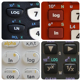

The common logarithm has a base of $10$. It is written as $\log$ (lowercase LOG). The natural logarithm has a base of $e$. It is written as $\ln$ (lowercase LN).

Graph Logarithmic Functions

We can also use the inverse function relationship to sketch graphs of logarithmic functions. Remember, with inverse function if the point $(x,y)$ is on the graph of $f$ then the point $(y,x)$ is on the graph of $f^{-1}$.

Use the figure below to help you graph $\log_2(x)$. As you move the blue point, the pencil will plot its inverse (in black).

You may want to verify that each of the following points is on the appropriate graph.

Point on $f(x)=2^{x}$	Point on $f^{-1}(x)=\log_{2}(x)$
$(0,1)$	$(1,0)$
$(1,2)$	$(2,1)$
$(2,4)$	$(4,2)$
$(3,8)$	$(8,3)$

Like exponential functions, the shape of the graph of a logarithmic function is controlled entirely by the value of the base $b$. Each base will have its own, slightly different graph. Use the following interactive figure to change the value of $b$ and analyze the behavior of the function.

Specifically, look for any of the 9 basic function properties. Click each property to check your observations.

Domain and Range

Domain includes all $x>0$, the Range is all real numbers.

y-intercept

Logarithmic functions never cross the y-axis, so there are no y-intercepts.

x-intercepts

All logarithmic functions have the same x-intercept of $x=1$.

Increasing, Decreasing, Constant

If $b>1$ the function is always increasing and represents logarithmic growth. Larger values of $b$ produce slower growth.

If $0 < b < 1$ the function is always decreasing and indicates logarithmic decay. The decay is greatest when $b$ is close to $1$.

The function does not exist when $b \leq 0$ or if $b=1$.

Maximums & Minimums

Since logarithmic functions are constantly increasing or decreasing they do not have any maximums or minimums.

Concavity

Concavity depends on the base. If $b>1$ the graph is concave down. If $0 < b < 1$ it will be concave up.

Asymptotes

No horizontal asymptotes exist, but the y-axis is a vertical asymptote.

Symmetry

Logarithmic functions do not have odd or even symmetry.

1:1

Yes, all logarithmic functions are 1:1. The inverse function would be the exponential function with the same base.

Understand How Logarithmic Functions Change

Every time we define a new function, we need to investigate the way it changes. Let's start by looking at the average rate of change $\frac{\Delta y}{\Delta x}$ over several intervals.

For convenience, we will use the common logarithm $\log(x)$ and, to simplify the calculations, we will choose intervals $[a, b]$ that have a width of $\Delta x=1$.

Interval	$\frac{\Delta y}{\Delta x} =\frac{f(b)-f(a)}{b-a}=\frac{\log(b)-\log(a)}{b-a}$
$[0.001, 1.001]$	$\frac{\Delta y}{\Delta x}=\frac{\log (1.001)-\log (0.001)}{1.001-0.001}=3.000$
$[1, 2]$	$\frac{\Delta y}{\Delta x}=\frac{\log 2-\log 1}{1-0}=0.301$
$[2, 3]$	$\frac{\Delta y}{\Delta x}=\frac{\log 3-\log 2}{3-2}=0.176$
$[3, 4]$	$\frac{\Delta y}{\Delta x}=\frac{\log 4-\log 3}{4-3}=0.125$
$[50, 51]$	$\frac{\Delta y}{\Delta x}=\frac{\log 51-\log 50}{51-50}=0.009$
$[100, 101]$	$\frac{\Delta y}{\Delta x}=\frac{\log 101-\log 100}{101-100}=0.004$

What do these values for $\frac{\Delta y}{\Delta x}$ in the table tell us about the common logarithm function? It appears that $\log(x)$ changes more when $x$ is small than it does when $x$ is large. In other words, the values of $\log(x)$ are further apart when $x$ is small, and closer together when $x$ is large. The difference quotient will help us understand why this happens.

Difference Quotient of Logarithmic Functions

In earlier chapters we saw that the difference quotient of a function, given by $D(x)=\frac{f(x+h)-f(x)}{h}$, is a function that describes how $f$ changes on any interval of length $h>0$.

Unlike power functions and exponential functions, it is very difficult to simplify the difference quotient of a logarithmic function by hand, so we will not attempt that.

However, since $D(x)$ is itself a function, we can take a look at its graph and see if it has any interesting properties.

It the figure below, the graphs of $f(x)=\log_{b}(x)$ and its difference quotient $D(x)$ are shown in black and in red, respectively.

We have fixed $h=0.001$, but the value of the base $b$ can change, allowing us to view the difference quotient for several different logarithms. Use the blue slider to change the value of $b$ and see if you recognize $D(x)$ as one of the basic functions from Chapter 1.

No matter which base is chosen, the graph of $D(x)$ always looks like the reciprocal function $1/x$. And the fact that $1/x$ is large when $x$ is small but small when $x$ is large confirms our earlier observation that logarithmic functions change rapidly when $x$ is small but that the rate slows down as $x$ increases.

Logarithmic Scales

When we plot values for $\log (x)$ on a number line it quickly becomes apparent that they are not evenly spaced. The smaller values are spread out while the larger values are more compressed.

If we use the logarithms as increments and relabel the axis we end up with something called a logarithmic scale.

Logarithmic scales have several applications, some of which will be covered in the next section. For now, we will use it like a ruler to measure lengths. In the process, we hope to uncover at least one property of logarithms.

Product Rule for Logarithms

We now turn our attention to some rather useful properties that deal with combining logarithms through addition and subtraction. Rather than deriving these properties by rewriting rules of exponents, we will attempt to discover some of them by using the logarithmic scale in this interactive figure. Keep in mind that since logarithms are exponents, we cannot expect the normal rules of addition to work.

Start by adding two logarithms. For instance, find $\log(3) + \log(5)$ by putting both $\log(3) $ and $\log(5)$ end-to-end on the log scale. Is the answer $\log(8)$ ? Experiment with other combinations to see if there is a pattern for addition.

Then move on to expressions like $\log(9) - \log(3)$. Since you are not given a bar for $\log(9)$ you might have to find multiple bars that add up to $\log(9)$ before you subtract $\log(3)$ away from them.

Use a calculator to check your work and make a note of your results before continuing.

Let's look closely at what you might have found from the interactive figure. This is what it would look like if you placed $\log(3) $ and $\log(5)$ end-to-end on the log scale.

Notice that the resulting bar lines up with $15$ on the log scale. We learn from this that $\log(3)+\log(5)=\log(15)$ or, in other words,

[ \log(3)+\log(5)=\log(3 \cdot 5) ]

If you try this with other values you will find that it is always true. The pattern is

[ \log(x)+\log(y)=\log(x \cdot y) ]

and is called the product rule.

Quotient Rule for Logarithms

Since addition always tells us something about subtraction, let's take another look at $\log(3) + \log(5)$.
We know that $\log(3)+\log(5)=\log(15)$, but what if we were to remove the $\log(5)$ from the figure above? The only thing left would be $\log(3)$. In other words, $\log(15)-\log(5)=\log(3)$. Since $\frac{15}{5}=3$ the pattern for subtraction is $\log(x)-\log(y)=\log\left(\frac{x}{y}\right)$ which is known as the quotient rule.

Power Rule for Logarithms

One of the most useful logarithm properties is called the power rule. Consider what happens when you add $\log(3)$ with another $\log(3)$.

Clearly $\log(3)+\log(3)=\log(9)$. And since $9=3^2$, this result can also be given as $\log(3)+\log(3)=\log(3^2)$.

But it is also proper to write $\log(3)+\log(3)=2 \cdot \log(3)$, just as we might write $5+5=2*5$.

Putting the two together we see that $\log(3^2)=2 \cdot \log(3)$. The general pattern is

[ \log x^{p}=p \cdot \log(x) ]

and will be used extensively throughout the rest of this chapter.

Properties of Logarithms

The properties we discovered are valid for all logarithms, no mater which base is used. We have listed them below in their general form. You are encouraged to use a calculator to check the given examples.

Identity	Formula	Example
Product Rule	[ \log_b (x \cdot y) = \log_b (x) + \log_b (y) ]	[ \ln(20) = \ln(4) + \ln(5) ]
Quotient Rule	[ \log_b \left(\frac{x}{y}\right) = \log_b (x) - \log_b (y) ]	[ \ln\left(\frac{10}{2}\right) = \ln(10) - \ln(2) ]
Power Rule	[ \log_b x^{p} = p \log_b (x) ]	[ \ln(2^{3}) = 3\ln(2) ]

Logarithms Throughout History

Tables of Logarithms

When John Napier discovered logarithms in 1614, he realized that with these logarithm rules, every operation could be converted to a simpler one.

The power rule changes multiplication into addition; the quotient rule turns division into subtraction; and the power rule replaces powers with multiplication.

The only tool needed to use these simplifications is a table of logarithmic values.

To illustrate how to use a table of logarithms, we'll examine a very simple case. Suppose we wanted to multiply $2$ and $3$. Rather than doing the multiplication, we look up the two logarithms in the table and calculate their sum: $\log(2) + \log(3) = 0.301 + 0.477 = 0.778$.

Next, we scan through the table until we find $0.778$. Lastly, we read the table backward to find the $x$ next to $0.778$. This value, $x = 6$ is the answer to our multiplication problem!

What we just did was a product rule: $\log(2)+\log(3)=\log(2 \cdot 3)$. And while our example was overly simple, the time saved when working with large numbers is tremendous since adding large numbers by hand is much faster than multiplying them.

Slide Rules

The rules of logarithms sped up calculations even more after the invention of slide rules.

Slide rules look similar to regular rulers except that the markings are not evenly spaced. Instead, the distances are proportional to the logarithms of the marked values. In essence, a slide rule is just two logarithmic scales, one placed on top of the other so they can slide back and forth.

Let's see how this works. Suppose you wanted to multiply $2 \cdot 3$. The first step is to slide the top scale to the right until the $1$ is above the $2$. Next move the hairline so that it is over the $3$ on the top scale. The answer, $6$, will be directly below on the lower scale.

Sliding the upper scale is a physical way to add logarithms and use the product rule. And while it may not be as precise as a table, it is very quick. Notice that no extra work is needed to calculate other multiples of $2$ because all the numbers on the top scale are now lined up with their multiples on bottom scale.

Looking Ahead

Modern calculators and computers have rendered both logarithm tables and slide rules obsolete.

However, the properties of logarithms that were developed in this section are valuable tools for solving exponential equations.

We will also return to logarithmic scales, but with a slight twist, at the end of the next section.